Technical details on the Stan programming language
Before we move onto further modeling in Stan, we need to understand a bit more about the language itself. This will help us both when constructing our Bernoulli and linear regression models in this exercise, and beyond.
Why use Stan?
Stan provides some advantages over previous probabilistic programming languages like BUGS (Bayesian inference Using Gibbs Sampling) and JAGS (Just Another Gibbs Sampler). This includes:
1. Computational efficiency - The time to run models is quicker, particularly for more complex models
2. Memory optimization - Stan uses only 1-10% of the memory required by BUGS/JAGS
3. Advanced language features - You can overwrite variables, and Stan implements vectorization
Vectorization allows you to perform operations on entire arrays or matrices at once, rather than using loops. In Stan, this not only makes code more readable but also significantly improves computational efficiency.
These advantages have made Stan particularly valuable for running complex hierarchical models, and models with many parameters.
For sampling, Stan uses the No U-Turn Sampler (NUTS) as it’s sampling method. You can see it’s efficiency versus two other MCMC methods (Metropolis and Gibbs sampling) in the graph below:
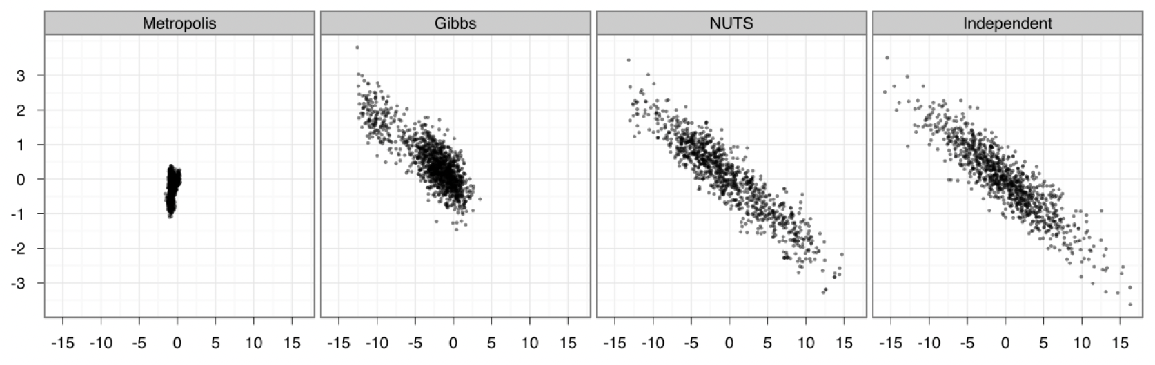
An example sampling distribution for various MCMC methods, with 1 million draws thinned to 1,000 (Metropolis, Gibbs) and 1,000 draws (NUTS) compared to the ground truth
Compared to Metropolis and Gibbs sampling, NUTS is able to perform a much better exploration of the parameter space, even with 1,000 times fewer draws! These samples ultimately look much more like the independent draws, which is a reference how the ideal sampling should look.
NUTS is an extension of Hamiltonian Monte Carlo (HMC) that automatically tunes the sampler’s parameters. It uses information about the gradient of the posterior distribution to make informed proposals for where to sample next, rather than the random walks used by Metropolis and Gibbs samplers.
You can learn more about Stan’s advantages in the “Selling Stan” discussion.

Variable types and declaration
Stan is a rather ‘un-intuitive’ programming language compared to R, Python or MATLAB, particularly due to its strict typing system and declaration rules.
Here is an overview of some of it’s key properties:
- Variables must be explicitly declared with both their type and scope before use
- All declarations must occur at the beginning of their respective blocks
- Types are static and strictly enforced throughout the program
Unlike flexible languages like R or Python, Stan strictly enforces type matching, with each variable having a type (static type; scalar, vector, matrix etc.).
Stan supports several basic types:
int: Integer valuesreal: Real (decimal) valuesvector: One-dimensional arrays of realsmatrix: Two-dimensional arrays of reals
Stan has two primary scalar types:
real: For continuous numeric values
data {
  real y;  // Unbounded continuous value
}int: For integer values
data {
  int n;  // Unbounded integer value
}
Stan also supports vector types for one-dimensional arrays of real numbers:
data {
  vector[3] v;  // Vector with 3 elements
}
and matrix types for two-dimensional arrays of real numbers:
data {
  matrix[3,2] m;  // Matrix with 3 rows and 2 columns
}
But types need to be correctly matched. The code below demonstrates that a vector cannot be assigned to a variable declared as a scalar type real:
// This works
real x;
x = 2.5;

// Whereas this would cause an error
real y;
y = [1, 2, 3];  // Can't assign vector to scalar
Stan allows you to constrain variables using lower and upper bounds. These constraints are particularly useful for ensuring counts are positive (lower=0) and restricting probabilities (lower=0, upper=1).
data {
   int<lower=1> m;                   // Integer ≥ 1
   int<lower=0,upper=1> n;           // Binary integer (0 or 1)
   real<lower=0> x;                  // Positive real number
   real<upper=0> y;                  // Negative real number
   real<lower=-1,upper=1> rho;       // Real number between -1 and 1
}
Stan also provides several types for handling multi-dimensional data such as vectors and matrices:
vector[3] a;                    // 3-element column vector
row_vector[4] b;               // 4-element row vector
matrix[3,4] A;                 // A is a 3×4 matrix, A[1] returns a 4-element row vector

// Constrained versions
vector<lower=0,upper=1>[5] rhos;      // 5-element probability vector
row_vector<lower=0>[4] sigmas;        // 4-element positive row vector
matrix<lower=-1,upper=1>[3,4] Sigma;  // 3×4 matrix with bounded elements
Global and local scope
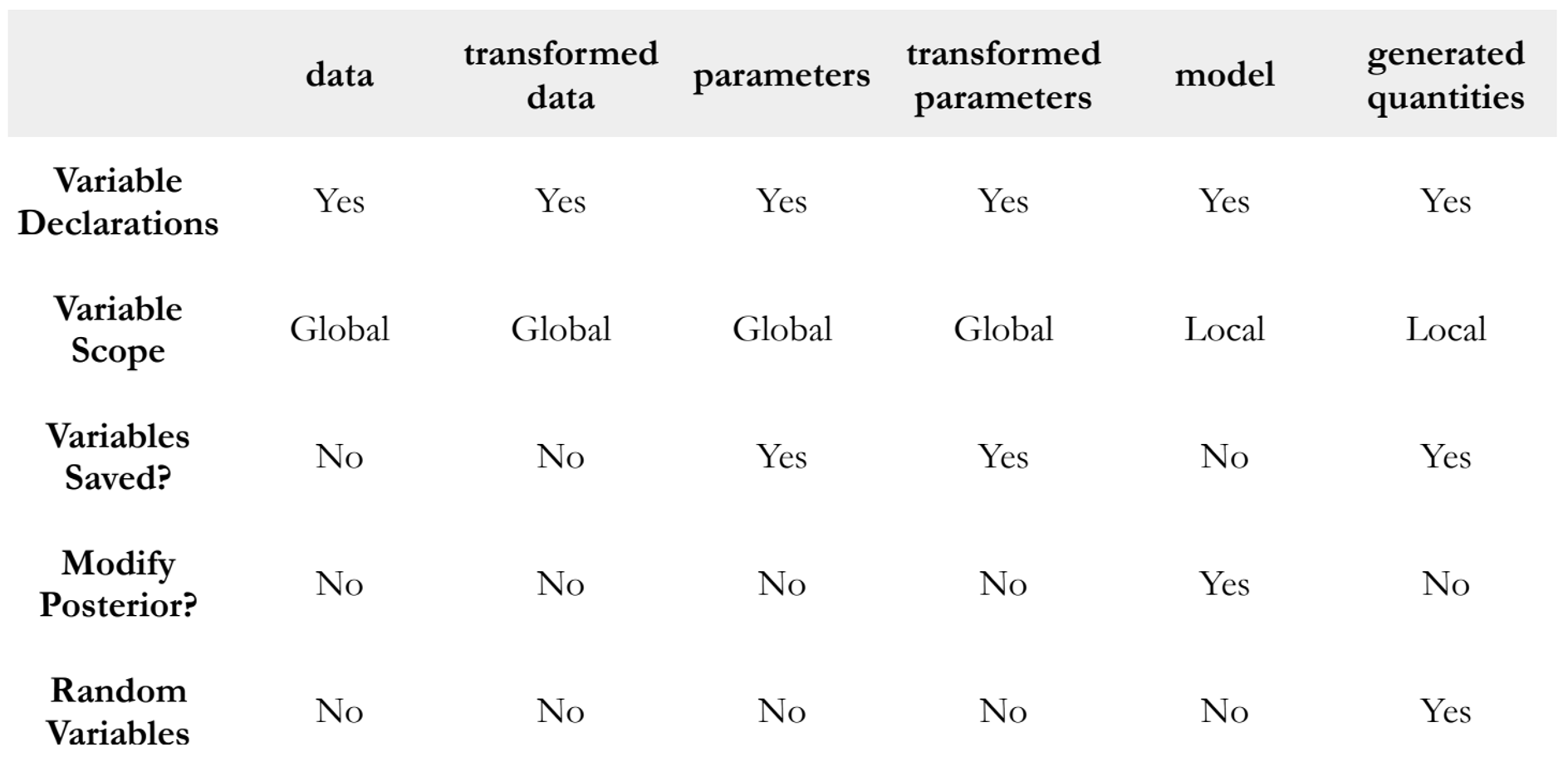
Each block in Stan has distinct properties that determine how variables can be used. While all blocks require variable declarations, their scope and behaviour varies:
The
data,transformed data,parameters, andtransformed parametersblocks have global scope, meaning these variables are accessible throughout the program.In contrast, variables in the
modelandgenerated quantitiesblocks have local scope. Variables declared within these blocks can only be accessed and used within this same block. They aren’t visible or usable in other parts of the Stan program.Only
parameters,transformed parameters, andgenerated quantitiesare saved in Stan’s output.The
modelblock is unique in that it can modify theposterior distribution, while thegenerated quantitiesblock is the only place where random variables can be generated.
Here’s some example Stan code demonstrating global versus local scope:
data {
  real x;      // Global: accessible everywhere
}

parameters {
  real theta;  // Global: accessible everywhere
}

model {
  real temp;   // Local: only exists in model block
  temp = x * 2;

  theta ~ normal(temp, 1);  // Can use both global (x, theta) and local (temp)
}

generated quantities {
  real pred;   // Local: only exists in generated quantities
  // temp not accessible here - it was local to model block

  pred = theta * x;  // Can use global variables (theta, x)
}
In this example, x and theta are global and accessible everywhere, while temp and pred are local variables that can only be used in their respective blocks.
Control flow
Stan also provides familiar control flow structures similar to R.
For example with if-else statements:
// Simple if
if (condition) {
    statement;
}

// If-else
if (condition) {
    statement;
} else {
    statement;
}

// If-else if-else
if (condition) {
    statement;
} else if (condition) {
    statement;
} else {
    statement;
}
And for-loops:
// Single for loop
for (j in 1:J) {
    statement;
}

// Nested for loops
for (j in 1:J) {
    for (k in 1:K) {
        statement;
    }
}Remember that unlike R, Stan requires semicolons (;) at the end of each statement within control structures!